FORECAST MODEL GRANULARITY: WHY TIME AND LOCATION MATTER IN LOAD FORECASTING

1. Introduction
In the previous articles, I discussed how future demand shapes grid investment and how different stakeholders use load forecasts for planning decisions. Before moving deeper into base load forecasting, it is important to first discuss one key methodological question:
At what level of detail should a load forecast be prepared?
This question is usually described as forecast model granularity.
In simple terms, granularity means the level of detail used in the forecast. A forecast can be developed at system level or feeder level. It can be annual, monthly, daily, hourly, or even sub-hourly. It can represent one large region, one load zone, one transmission node, one distribution substation, or one customer class.
This matters because a forecast is only useful if its level of detail matches the planning question. A forecast that is good enough for long-term resource planning may not be detailed enough for distribution planning. Similarly, a feeder-level forecast may be too detailed for market-wide adequacy studies unless it is properly aggregated.
The ESIG report highlights that modern load and DER forecasting increasingly requires both temporal granularity and geographic granularity to capture changing demand patterns, DER adoption, electrification, and localized load growth [1].
2. What Is Forecast Model Granularity?
Forecast model granularity can be understood in two dimensions:
Temporal granularity
This refers to how demand is represented over time, e.g.
annual peak demand
monthly energy demand
daily load profile
hourly load profile
8,760 hourly time-series forecast
Spatial granularity
This refers to where demand is represented in the network, e.g.
system level
load zone level
transmission node level
distribution substation level
feeder level
customer or meter level
Both dimensions are important.
A planner may know the total demand growth of a region, but if the forecast does not show where the demand appears, it may miss local constraints. Similarly, a planner may know the annual peak demand, but if the forecast does not show when the demand appears, it may miss ramping needs, midday minimum load, evening peaks, or seasonal operating stress.
3. Why Temporal Granularity Matters
Traditional long-term load forecasts often focused on annual energy and annual peak demand. This was useful when electricity demand was relatively predictable and the system was dominated by centralized generation.
However, modern demand is becoming more dynamic.
Electric vehicles may charge outside traditional peak periods. Rooftop PV may reduce midday net load. Batteries may shift demand between hours. Heat pumps may create new winter peaks. Data centers may introduce large and relatively flat demand profiles. Extreme weather may create short-duration but high-impact demand events.
This is why hourly forecasting is becoming more important.
An 8,760 hourly forecast represents every hour of the year. It allows planners to see not only the annual peak, but also:
hourly load shape
seasonal variation
minimum load conditions
evening ramps
non-coincident local peaks
DER impact on net load
EV charging behaviour
weather-driven demand patterns
This does not mean every study always needs an 8,760 forecast. It means the time resolution should be selected based on the planning purpose as shown in below table.
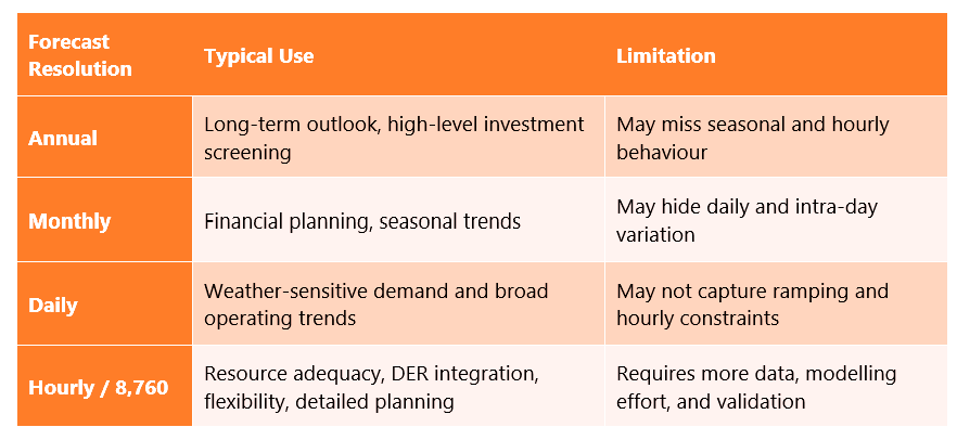
The key point is simple: as the grid becomes more dynamic, time resolution becomes more important.
4. Why Spatial Granularity Matters
Spatial granularity is equally important.
A system-level forecast may show that the overall grid has enough capacity, but this does not mean every local area is secure. A specific substation, feeder, industrial zone, data center cluster, or EV charging corridor may become constrained even if the wider system appears adequate.
This is especially important for:
EV fast-charging hubs
data center clusters
industrial electrification
rooftop PV concentration
behind-the-meter BESS
heat pump adoption
new urban developments
distribution-level load pockets
For example, a 500 MW increase in demand spread across a large region may be manageable. But the same 500 MW concentrated near one transmission node or one group of substations may require major reinforcement.
This is why modern planning increasingly needs forecasts that can move between different geographic levels:
system forecast
load zone forecast
transmission node forecast
substation forecast
feeder forecast
customer class forecast
The forecast must be detailed enough to reveal the planning issue.
5. The Trade-Off: Detail Versus Complexity
Higher granularity improves visibility, but it also increases complexity.
A highly detailed forecast needs better data, more assumptions, stronger modelling capability, and more validation. For example, an hourly forecast at feeder level over a 20-year horizon creates a large amount of data. A customer-level DER adoption forecast may be very detailed, but it may also carry significant uncertainty.
Therefore, planners must balance:
accuracy
data availability
modelling complexity
computational effort
planning horizon
stakeholder needs
decision impact
The objective is not to make every forecast as detailed as possible. The objective is to make the forecast fit for purpose.
A financial planning forecast may be acceptable at customer-class or service-territory level. A transmission planning forecast may need allocation to transmission nodes. A distribution planning forecast may need substation or feeder-level detail.
6. Aggregation and Disaggregation
Another important methodological concept is the movement of forecasts between different levels of the grid.
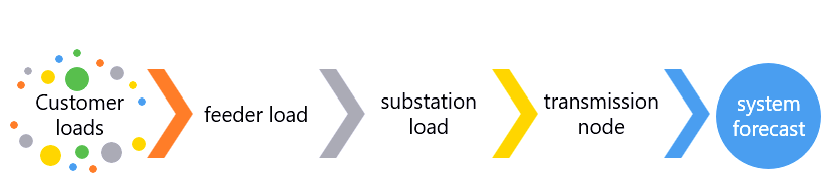
Aggregation means combining lower-level data into a higher-level forecast.
For example:
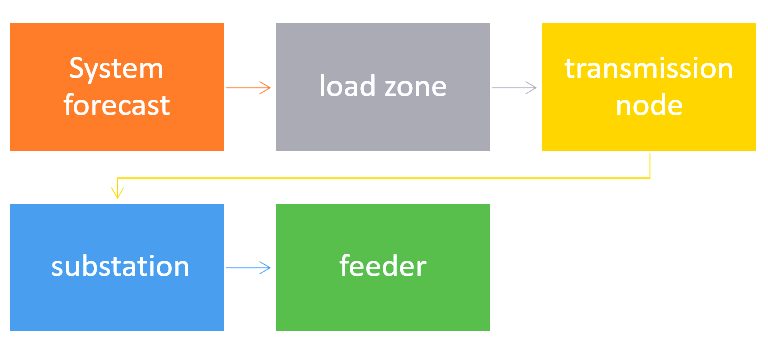
Disaggregation means allocating a higher-level forecast down to more detailed grid locations.
For example:
Both approaches are used in planning.
However, both can create errors if not handled carefully. A top-down system forecast may miss local load pockets. A bottom-up distribution forecast may overestimate total system demand if diversity and coincidence are not properly considered.
This is why reconciliation is important. Planners need to check whether system-level, transmission-level, and distribution-level forecasts are consistent enough for the intended planning use.
7. Matching Granularity with the Planning Use Case
A good forecasting methodology starts by asking:
What decision will this forecast support?
Different planning studies need different forecast resolution.
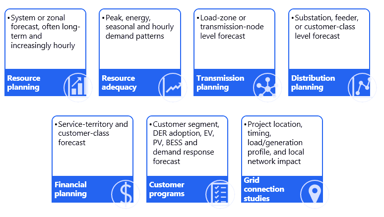
This shows why a single forecast cannot answer every planning question. The same demand outlook may need to be represented differently depending on whether the question is about adequacy, congestion, voltage, system strength, distribution reinforcement, tariff design, or grid connection.
8. Why This Comes Before Base Load Forecasting
Before developing a base load forecast, planners should first understand the required forecast resolution.
This is important because the base load forecast may be built differently depending on the intended use. A system-level base forecast may rely on economic, demographic, and weather-normalized trends. A feeder-level forecast may require SCADA, AMI, customer connection data, and local development information.
Therefore, the correct sequence is:
Define the planning use case
Select the temporal and spatial granularity
Collect and validate historical data
Develop the base load forecast
Add known new customer loads
Add DERs, electrification, and flexible demand
Apply scenarios and uncertainty analysis
Produce the final planning forecast
This sequence helps avoid one common problem: developing a forecast first and only later discovering that it does not have the right resolution for the planning study.
9. Key Takeaway
Forecast model granularity is not just a modelling detail. It is a planning decision.
If the forecast is too broad, it may hide local constraints. If it is too coarse in time, it may miss ramping needs, minimum load conditions, or non-coincident peaks. If it is too detailed without good data, it may create false confidence.
The key message is simple:
A load forecast must match the planning question. The right level of time and location detail is essential for reliable planning, efficient investment, and effective grid connection decisions.
In the next article, the discussion can move into the components of the long-term load and DER forecasting process, including top-down and bottom-up approaches, base load forecasting, known new customer loads, DERs, electrification, uncertainty, and scenario planning.
Reference
[1] Energy Systems Integration Group, Long-Term Load and DER Forecasting, A Report by the Energy Systems Integration Group’s Long-Term Load and DER Forecasting Task Force, Aug. 2025.